A developer deploys a state-of-the-art NVIDIA A100 GPU, expecting a massive leap in inference throughput, only to find that the actual execution speed barely budges. The hardware spec sheet promises teraflops of compute power, yet the real-world latency remains stubbornly high. This gap between theoretical peak performance and actual runtime is rarely a failure of the silicon; instead, it is almost always a symptom of code-level bottlenecks where the GPU spends more time waiting for instructions than actually performing calculations. To bridge this gap, engineers must move beyond simple timers and dive into the granular execution flow using the torch.profiler module.
Quantifying the Gap with torch.profiler and Perfetto
Analyzing performance on an NVIDIA A100-SXM4-80GB requires a dual-pronged approach to data extraction. When running a profiling script like 01_matmul_add.py, the torch.profiler module generates two distinct artifacts that serve different diagnostic purposes. The first is a text-based profiler table, which provides a quantitative audit of every event triggered during the execution window. This table lists the number of calls and the precise time spent on both the CPU and GPU for each operation. By correlating the # of Calls column with the time metrics, developers can pinpoint which specific operators are consuming the most resources or being called with inefficient frequency.
The second artifact is a JSON trace file designed for the Perfetto UI, a high-performance visualization tool. While the text table provides the what, the JSON trace provides the when. By uploading this file to Perfetto, the execution timeline is split into parallel lanes for the CPU and GPU. The length of the bars represents the duration of an event, and their vertical stacking reveals the call hierarchy. The most critical insight in this view is the empty space between the CPU and GPU lanes. These gaps represent idle time or kernel dispatch latency, where the GPU is essentially dormant while the CPU struggles to prepare the next command. To get a clean reading, analysts must carefully isolate the steady-state execution phase and strip away the noise generated during the initial environment setup.
To distinguish between a function that is slow because of its own logic and one that is slow because it calls other expensive functions, the profiler tracks Self CPU/CUDA and CPU/CUDA Total metrics. Self time measures the duration spent exclusively within that specific event, excluding any child calls. Total time, conversely, aggregates the duration of the event and every sub-operation it triggers. For instance, a matmul_add function's CPU Total time includes the overhead of the function wrapper plus the time spent in the underlying linear algebra kernels. For those needing to generate direct links to their trace analysis, the following command is used:
uvx trace-util traces -b tracesNavigating the Perfetto interface requires using the W, A, S, and D keys to pan and zoom through the timeline. By contrasting the CPU lane's event sequence with the GPU lane's kernel execution, developers can visualize the exact moment a kernel is submitted and the subsequent delay before the GPU actually begins processing. This interval is the primary metric for analyzing launch overhead.
The Shift from Overhead-Bound to Compute-Bound Execution
The true nature of GPU inefficiency becomes apparent when comparing small-scale operations to large-scale workloads. In a test using 64x64 matrices, the discrepancy between hardware capability and actual speed is jarring. Profiling reveals that the execution time of the GPU kernel, specifically ampere_bf16_s16816gemm, accounts for less than 1% of the total CPU processing time. This is a classic overhead-bound state. In this scenario, the time required for the CPU to prepare the kernel, manage the driver stack, and launch the operation outweighs the actual computation time. The GPU is effectively a Ferrari stuck in a school zone; it possesses immense power, but it spends the vast majority of its time idling, waiting for the CPU to give it the green light. Increasing the GPU's clock speed or adding more cores in this state provides zero performance gain because the bottleneck is not the compute, but the orchestration.
However, as the matrix size increases, the bottleneck shifts. When the workload is scaled up, the time the ampere_bf16_s16816gemm kernel spends performing actual calculations begins to exceed the CPU's launch time. The system transitions into a compute-bound state. In this phase, the fixed cost of the CPU launch becomes a negligible fraction of the total execution time, and the GPU's raw throughput becomes the primary determinant of speed. This transition proves that maximizing GPU utilization is not about the speed of the hardware, but about the volume of work assigned per call. Ensuring that the operation size is large enough to dwarf the launch overhead is the only way to unlock the latent performance of the A100.
This analysis also uncovers a hidden latency known as the dead window. Profiling shows a gap of approximately 228µs from the moment record_function("matmul_add") is entered until the kernel is actually dispatched. This delay is caused by one-time costs including workspace allocation, cuBLAS heuristic calculations to determine the fastest algorithm for the given matrix size, and lazy loading of modules. If these are included in a benchmark, the results are skewed, masking the true performance of the model. To solve this, a warmup strategy is mandatory. The PyTorch profiler allows for a scheduled approach consisting of a wait phase to settle the system, a warmup phase to trigger initializations without recording, and an active phase for actual data collection. While this removes the 228µs one-time cost, it does not eliminate the structural offset of roughly 2.5ms that exists between CPU submission and GPU start, which is an inherent characteristic of the driver and hardware interface.
For engineers optimizing LLM inference, these findings are critical. LLM generation often involves repeated small matrix multiplications, especially during the decoding phase. If the system remains in an overhead-bound state, the GPU will be chronically underutilized, and the tokens-per-second rate will plateau regardless of the hardware. The solution lies in batching. By grouping multiple requests or expanding the operation scale, the system is forced into a compute-bound state, reducing the relative impact of the CPU launch overhead and significantly increasing throughput.
Ultimately, the goal is to eliminate unnecessary CPU-GPU synchronization points that force the GPU to wait. A rigorous warmup phase and a structural redesign to minimize kernel launch frequency are more effective than hyperparameter tuning. The data provided by the PyTorch profiler proves that inference efficiency is not determined by algorithmic complexity, but by the precision with which data flow congestion is removed from the pipeline.